How We Fine-Tuned an Embedding Model to Solve Retail Misclassification: A Complete Guide (Code Included)

In this guide, we will fine-tune a leading MTEB (Massive Text Embedding Benchmark ) embedding model specifically for retail applications. Our aim was to optimise the model for three critical use cases:

1. Product Similarity Matching – To identify and group semantically similar products.
2. Taxonomy Standardisation – To fix inconsistencies in product categorisation during inventory migration.
3. Inventory Migration Optimisation – To simplify the transition of products across platforms with differing taxonomies.

As with any industry, retail is no easy. Platforms have their own rules for categorising products. For instance, one platform might list a product as “Wireless Earbuds”, while another platform calls the same item “Bluetooth Headphones”. Even though they refer to the same product type, their differing taxonomies create conflicts during inventory migration.

The result? Inconsistent product classifications across platforms, difficulty in grouping similar items, and errors that slow down operations. Worse, these issues directly impact your bottom line:

• Poor product search results frustrate customers, causing lost sales.
• Manually fixing taxonomies takes time and resources, increasing costs.
• Inventory migrations fail to run smoothly, disrupting your operations.

And as your catalog grows or new platforms are added, these inconsistencies multiply, making the issue even harder to manage.

What’s Missing in Traditional Solutions?

Most existing systems rely on manual fixes, keyword-based models, or rigid rules that fail to grasp the nuances of product data. For example:

• They can’t recognize that “Biotin Shampoo” and “Volumizing Conditioner” belong in the same Hair Care category.
• Worse, they might pair “Dark Chocolate” with “Chocolate Creme Body Lotion” simply because they share a word in their description.

This lack of contextual understanding creates inefficiencies and prevents businesses from delivering the seamless experiences that today’s customers demand. The solution?

To solve this, we turned to embedding models. These models capture the semantic similarities—so when we talk about “wireless earbuds” and “Bluetooth headphones,” the model understands they belong to the same category, even if they are labeled differently across systems.

Access the Code and Model
You can find the code and fine-tuned model used in this guide here:
GitHub
HuggingFace Model

Why Fine-Tuning Is Necessary in Retail

Pre-trained embedding models are excellent at general-purpose semantic understanding. They fall short when handling domain specific challenges like retail, where unique taxonomy structures, product descriptions, and customer behaviours come into play.

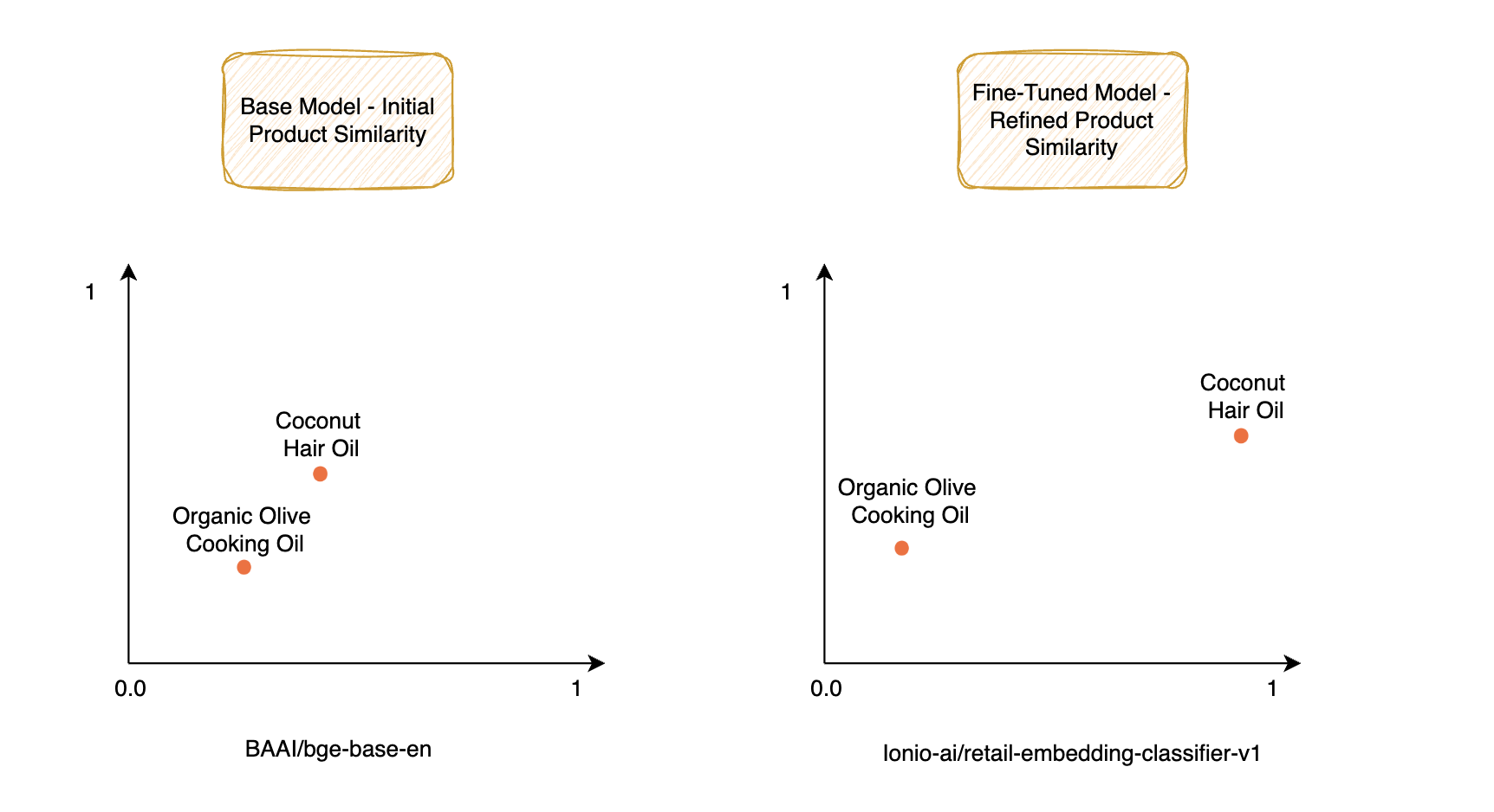
A general-purpose model doesn’t understand the nuances of product similarities or how retail-specific terms like "Coconut Hair Oil" and "Intense Hair Repair Shampoo" belong to the same category “Hair Care”, yet differ subtly in function.

Products belonging to a same brand may or may not be of the same category. In some cases, even if the label of a product is similar to another, it could be that they both have different descriptions and overall different use-case. You would not want such mishaps to happen, right?

In 2023, U.S. consumers returned $743 billion worth of merchandise, which made up 14.5% of total sales, according to the National Retail Federation. This is the direct result of poor product descriptions and misclassifications. When products are mislabeled or miscategorised, customers end up with items that don’t meet their expectations, leading to returns.

And returns are costly.

They increase shipping costs, waste valuable resources, and damage customer trust.

This is where product embeddings come into play.

At a high level, embeddings are a way to represent products in a format that computers can easily understand: vectors in a high-dimensional space. Each product is mapped to a point in this space based on its characteristics, such as category, description, and other attributes. The closer two vectors are, the more semantically similar the products are.

We analysed the dataset of a leading retail business and fine-tuned our model on its dataset, which contains over 11 categories and 90 subcategories. These categories span various types of products, from beauty and hygiene items to kitchen essentials and household goods.

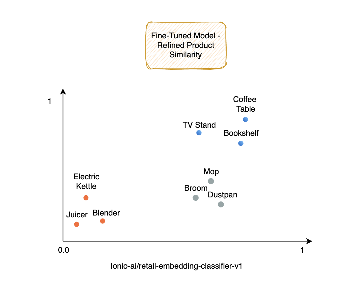
For instance, consider the products in our dataset:

• Electric Kettle, Juicer and Blender all belong to the same category of ‘Kitchen Appliances’, thus appearing close to each other in the vector space
• Likewise, products from ‘Home Furniture’ like the Coffee Table, TV Stand and Bookshelf are closely related to each other.
• ‘Cleaning supplies’ like a Mop, Broom and Dustpan get closely identified by our fine-tuned model since they come under the same category.

Even if their names, forms, or specific sub-categories differ, embeddings bring products closer in the semantic space when they share functional similarities, resulting in more accurate categorisations and better recommendations.

Dataset Manipulation

When fine-tuning an embedding model, the dataset (sourced from BigBasket’s complete product list) plays a crucial role in teaching the model to understand the nuances of your specific use case. In our case, we worked on fine-tuning a model for product similarity and classification. To achieve good results, we had to enhance and manipulate the dataset to make it suitable for the task.

Let me walk you through the data manipulation process step by step, including examples and code snippets.

Why the Original Dataset Wasn't Sufficient (for Fine-Tuning the Model) ?

We utilised Sentence Transformers to fine-tune our embedding model. The original dataset consisted of 27,555 rows, representing individual products with attributes like name, category, and description. However, this wasn’t sufficient for fine-tuning an embeddings model.

You may wonder why?

The dataset lacked the essential pairwise context that an embedding model requires for learning product relationships. No embedding model can learn from isolated points. It looks for some relationship or dependency for it to understand the pattern.

Without this pairwise data, the model wouldn’t learn how one product compares to another in terms of similarity or dissimilarity. It would only be able to understand individual product descriptions, missing the key relationships that define product categorisation and similarity.

For example, the model would struggle to learn how two different "Hair Care" products are related or why a "Shampoo" is more similar to another "Shampoo" than to a "Chocolate Bar.”

To address this, we:

1. Created Matched Combinations: Paired products within the same subcategory to highlight similarities.
2. Created Mismatched Combinations: Paired products from different subcategories to represent dissimilarities.
3. Expanded the dataset to over 218,000 records, ensuring a balanced representation of matched and mismatched pairs.

Also we needed the dataset to fit a specific format. Sentence Transformers requires a pairwise comparison of products, so the model can learn how similar or dissimilar two products are. This requires a dataset in a specific format, such as pair, pair-class, pair-score, or triplet. Specifically, we decided on the pair-score format, which consists of two product descriptions and a similarity score between them.

This meant that the original dataset had to be transformed into product pairs, some matched (similar products) and some mismatched (dissimilar products). Additionally, we needed to assign similarity scores to these pairs to guide the fine-tuning of the model.

Step 1: Generating Matched Combinations

What are Matched Combinations?

Matched combinations represent pairs of products that are closely related and belong to the same subcategory. These combinations are used to teach the model about similarities between items, helping it learn to cluster related products in the embedding space.

• Products within the same subcategory share common traits but aren’t identical.
• For instance, two shampoos might have different ingredients and descriptions but serve the same purpose (e.g., "Hair Care").
• By pairing such items, the model learns to assign similar embeddings to related products, which is essential for tasks like recommendation systems or product grouping.

How It Works

For each product in a subcategory, we paired it with up to 5 other products from the same subcategory. If fewer than 5 products were available, we used all remaining products. The goal was to create as many meaningful pairs as possible to capture product similarity.

Code Implementation

Here’s the code we used to generate matched combinations:

def generate_combinations(df):
    combinations = set()  
    for sub_category, group in df.groupby('sub_category'):
        products_combined = group[['product', 'combined']].set_index('product')
        products = products_combined.index.tolist()
        for i in range(len(products)):
            for j in range(i + 1, min(i + 6, len(products))):  # Pair with the next 5 products
                prod_1 = str(products_combined.loc[products[i], 'combined'])
                prod_2 = str(products_combined.loc[products[j], 'combined'])
                if prod_1 != prod_2:
                    combinations.add(tuple(sorted([prod_1, prod_2])))
    combination_df = pd.DataFrame(list(combinations), columns=['product_1', 'product_2'])
    return combination_df

‍The function generated 134,917 matched pairs. Each row represents two products that belong to the same subcategory.

Let’s consider the "Hair Care" subcategory. Some products in this subcategory might include:

• "Aloe Vera Shampoo - Gentle cleanser for all hair types."
• "Herbal Hair Oil - Nourishes and strengthens hair."
• "Garlic Oil Capsule - Promotes hair growth naturally."

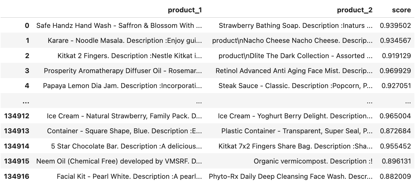
Here, the similarity score is set between 0.87 and 0.96, reflecting that the products are related but not identical.

Step 2: Generating Mismatched Combinations

What are Mismatched Combinations?

Mismatched combinations pair products from different subcategories. These pairs are vital for teaching the model about inter-category dissimilarities—helping it understand how products differ when they belong to separate subcategories.

• While matched combinations teach the model what’s similar, mismatched combinations teach it what’s not similar.
• For example, pairing a shampoo from "Hair Care" with a chocolate bar from "Snacks" shows the model that these items are entirely different, creating a clear boundary in the embedding space.

How It Works

For each product, I randomly sampled 3 products from different subcategories to create mismatched pairs. This ensured a diverse representation of dissimilar products in the dataset.

Code Implementation‍

import pandas as pd
import random

def generate_mismatched_combinations(df):
    mismatched_combinations = []
    other_sub_category_products = {sub_cat: df[df['sub_category'] != sub_cat] for sub_cat in df['sub_category'].unique()}

    # Iterate through each product
    for idx, row in df.iterrows():
        product = row['product']
        product_combined = str(row['combined'])
        product_sub_category = row['sub_category']
        other_products_df = other_sub_category_products[product_sub_category]
        sampled_other_products = other_products_df.sample(n=min(3, len(other_products_df)), random_state=42)

        for _, other_row in sampled_other_products.iterrows():
            other_product_combined = str(other_row['combined'])
            mismatched_combinations.append((product_combined, other_product_combined))
    mismatched_combination_df = pd.DataFrame(mismatched_combinations, columns=['product_1', 'product_2'])
    return mismatched_combination_df

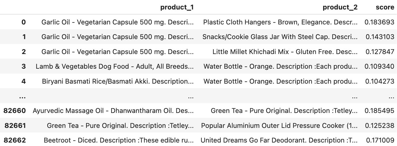
This process generated 82,665 mismatched pairs.

Let’s consider products from two different subcategories, "Hair Care" and "Snacks", similarity score here is set between 0.12 and 0.24, indicating that these products are dissimilar.

Why This Manipulation Was Crucial

By creating matched and mismatched pairs, I ensured the dataset:

1. Captured intra-category similarities through matched combinations.
2. Represented inter-category dissimilarities through mismatched combinations.
3. Provided a clear label structure for training the model using loss functions like CosineSimilarityLoss or CoSENTLoss.

Final Dataset Format

After generating both matched and mismatched combinations, we switched to a pair-score dataset format. This format includes:

1. product_1: Name + description of the first product.
2. product_2: Name + description of the second product.
3. similarity_score: A numeric score between 0 and 1.

We had two main parts in the dataset: one containing matched combinations (where product pairs were similar) and the other containing mismatched combinations (where the pairs were not similar). The task was to combine these two parts to form a unified dataset:

combined = pd.concat([combination_df, mismatched_combination_df], ignore_index=True)

We used pd.concat() to concatenate the two DataFrames, ensuring that the indices were reset (ignore_index=True).

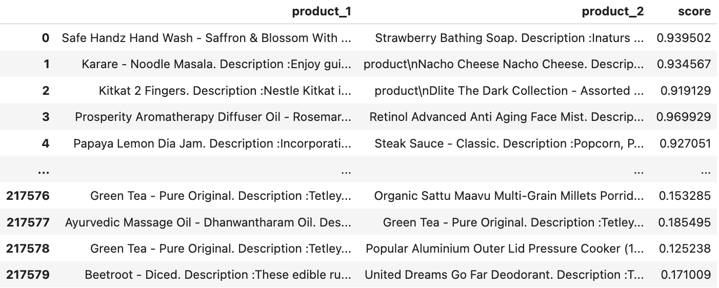
This format allowed us to fine-tune the model using loss functions like CosineSimilarityLoss, which require a pair-score dataset.

To handle the large dataset efficiently, we ran all manipulations on a RunPod A100 GPU. This setup allowed me to scale the dataset to 218,000 rows without significant performance bottlenecks.

How We Did It: The Fine-Tuning Process

This section will guide you through every detail of the fine-tuning process, explaining why each step is necessary, what each action accomplishes, and how it contributes to achieving the desired outcome.

Here, we fine-tuned the BAAI/bge-base-en model using a dataset of retail product information to enhance its understanding of product similarity.

Converting to Hugging Face Dataset:

from datasets import Dataset
hf = Dataset.from_pandas(combined)

Since the Sentence-Transformers library requires the data in a specific format, we converted the combined pandas DataFrame into a Hugging Face Dataset:

This step is necessary because the Sentence-Transformers framework leverages the Hugging Face Datasets library for efficient data handling during training.

Once the dataset was prepared, the next step was to split it into training, evaluation, and test sets. This ensures that the model can be evaluated on unseen data during the training process. We performed an 80-20 train-test split and further divided the test set into evaluation and validation setsFinally, we saved these splits to disk, ensuring that we can load them back efficiently during training.

1. Setting up the Model:

We chose the BAAI/bge-base-en model, which is a variant of BERT optimised for understanding English sentence representations. The model is suitable for our task as it was pre-trained on large-scale English data and can be fine-tuned to specific tasks like product similarity.‍

from sentence_transformers import SentenceTransformer

model = SentenceTransformer("BAAI/bge-base-en", trust_remote_code=True)

The trust_remote_code=True flag is used because the model is hosted on the Hugging Face Model Hub, and we are trusting that the code from the model repository is safe to execute.

2. Setting the Loss Function:

For this fine-tuning task, we chose the Cosine Similarity Loss. This is the most appropriate choice for tasks where we want the model to learn semantic similarity between pairs of sentences. The loss function minimises the cosine distance between the embeddings of matching product pairs, while increasing the distance for non-matching pairs.‍

from sentence_transformers.losses import CosineSimilarityLoss

loss = CosineSimilarityLoss(model)

Other loss functions are available, such as SoftmaxLoss and TripletLoss, but CosineSimilarityLoss is generally the most effective for tasks involving similarity learning, especially when the task is comparing sentence embeddings (e.g., product descriptions).

3. Configuring Training Arguments:

The most result oriented and core step is to step up accurate args for any training process. To fine-tune the model, we needed to define the training parameters, including the number of epochs, learning rate, batch size, and other aspects of the training loop. These settings were specified using the SentenceTransformerTrainingArguments class.

from sentence_transformers import SentenceTransformerTrainer
from sentence_transformers.training_args import SentenceTransformerTrainingArguments
from sentence_transformers.training_args import BatchSamplers

args = SentenceTransformerTrainingArguments(
    output_dir="bge-small-ft-retail",
    num_train_epochs=3,
    per_device_train_batch_size=64,
    per_device_eval_batch_size=64,
    learning_rate=2e-5,
    warmup_ratio=0.1,
    fp16=False,
    bf16=True,  # Set to True if your GPU supports BF16
    eval_strategy="steps",
    eval_steps=100,
    save_strategy="steps",
    save_steps=100,
    save_total_limit=2,
    logging_steps=100,
    run_name="bge-small-ft-retail",
)

Explanation of Key Parameters:

• num_train_epochs: Defines the number of complete passes through the dataset during training. We set it to 3, meaning the model will see the data three times.
• per_device_train_batch_size: The number of training examples in each batch. A batch size of 64 was chosen to balance memory usage and training speed.
• learning_rate: Controls how much the model weights are updated during each training step. A smaller learning rate like 2e-5 is chosen to fine-tune the model gently.
• warmup_ratio: Fraction of total steps to perform learning rate warm-up. This helps in stabilizing training in the initial stages.
• fp16 and bf16: These control the use of 16-bit floating point precision for training, which can speed up training and reduce memory usage. We set bf16=True, as the training was conducted on an A100 GPU, which supports BF16.
• eval_strategy and eval_steps: Set the evaluation frequency during training. In this case, the model is evaluated every 100 steps.
• save_strategy and save_steps: These define how frequently to save model checkpoints. We saved the model every 100 steps.
• logging_steps: This defines how frequently training statistics (like loss) are logged. Here, we log every 100 steps.

4. Training the Model:

With the training arguments and the loss function set, we initialised the SentenceTransformerTrainer:

trainer = SentenceTransformerTrainer(
    model=model,
    args=args,
    train_dataset=train_dataset,
    eval_dataset=eval_dataset,
    loss=loss,
)

‍Finally, we started the training process with:‍‍

trainer.train()

Training Logs:

The logs provided during training showed how both the training loss and validation loss evolved. Here’s a sample of what the logs looked like after training for three epochs:‍

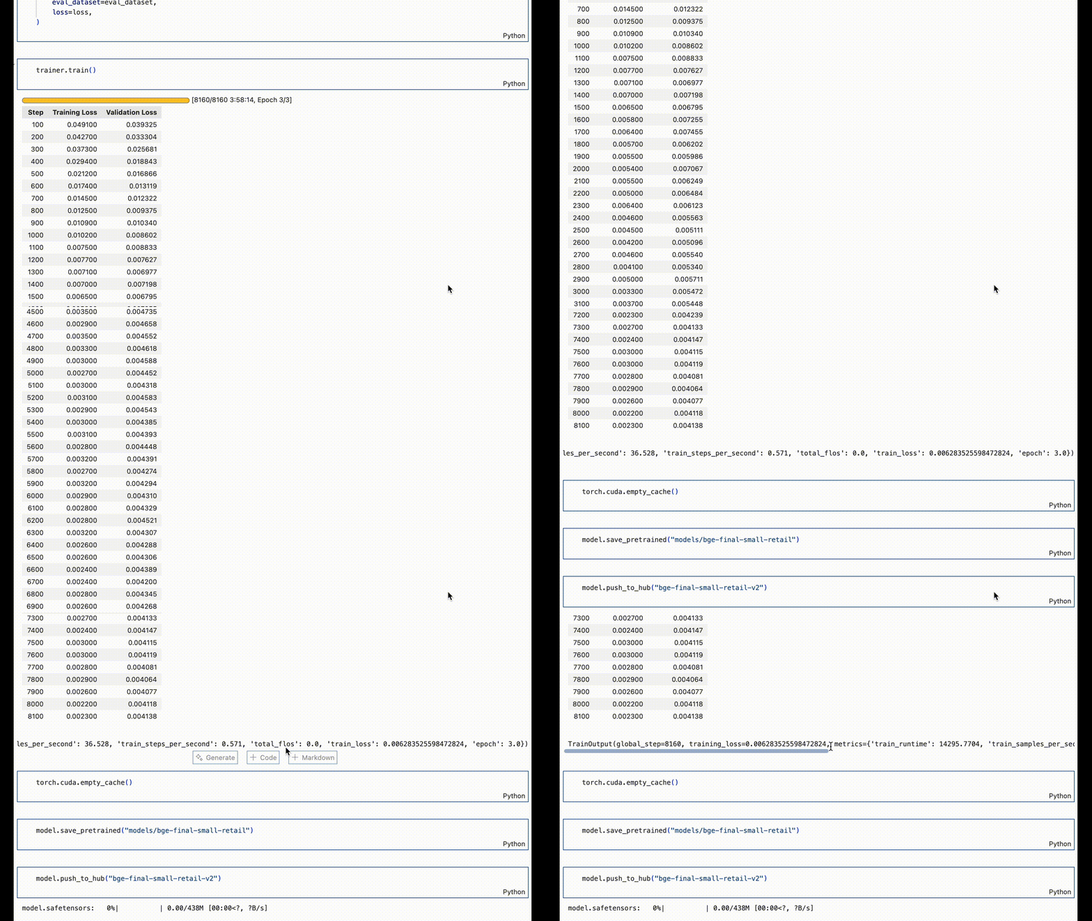
‍‍We can see that as the training progressed, both the training loss and validation loss decreased, indicating that the model was learning effectively.

7. Monitoring with Weights and Biases (WandB):

To monitor the training process in real-time, we used Weights and Biases (WandB). By installing and logging into WandB, we could track metrics like loss, learning rate, and other relevant information during training. This is especially useful for debugging and ensuring that training is proceeding smoothly.‍

pip install wandb
wandb.login()

Training Loss (train/loss)

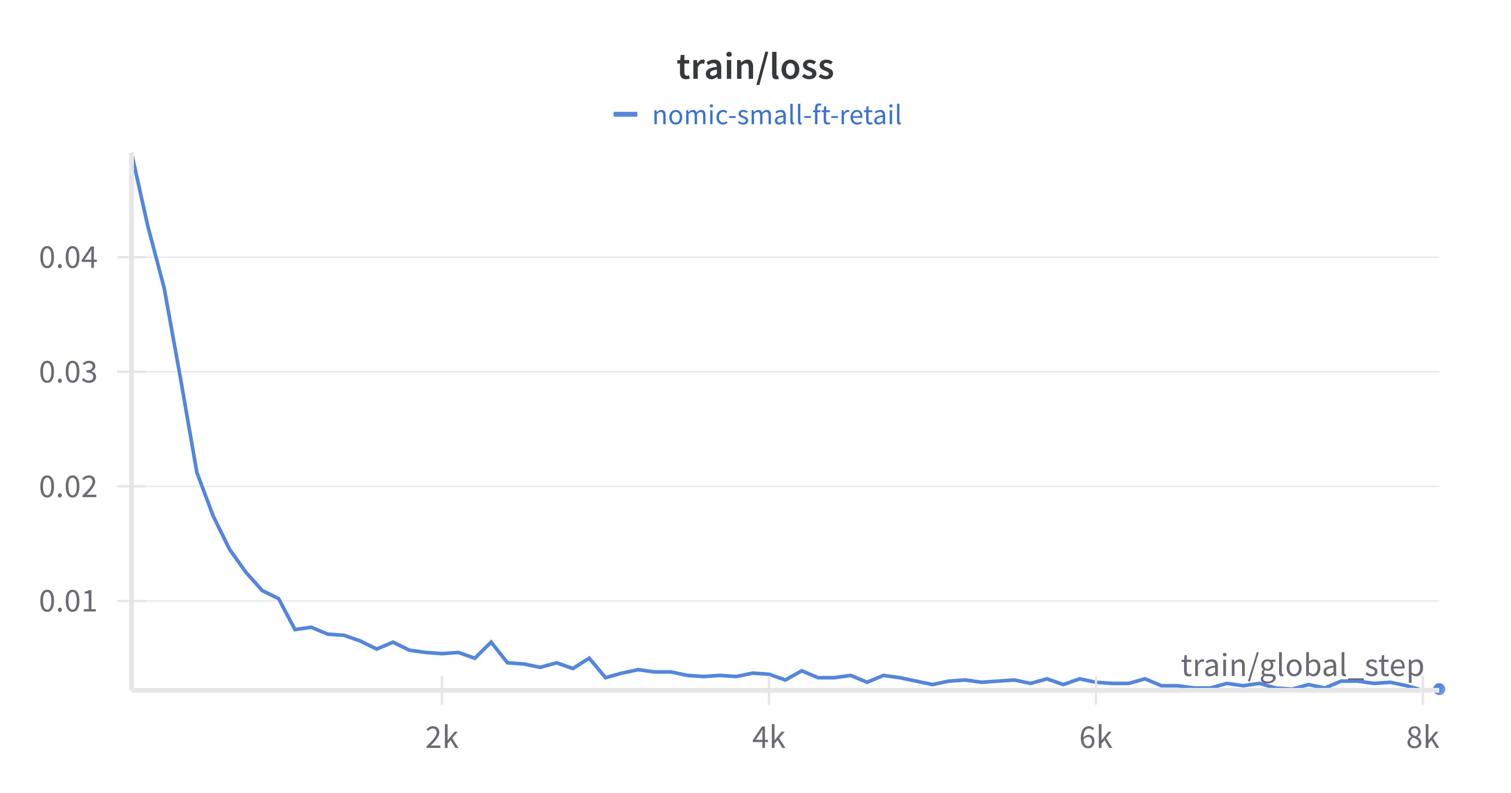
This chart shows how the model's loss decreased over time, indicating its ability to minimize errors during training.

• A steady decline in training loss confirms that the model is learning effectively.
• Highlights the convergence behaviour of the model.

Learning Rate (train/learning_rate)

The wandb plot depicts the learning rate schedule used during training.

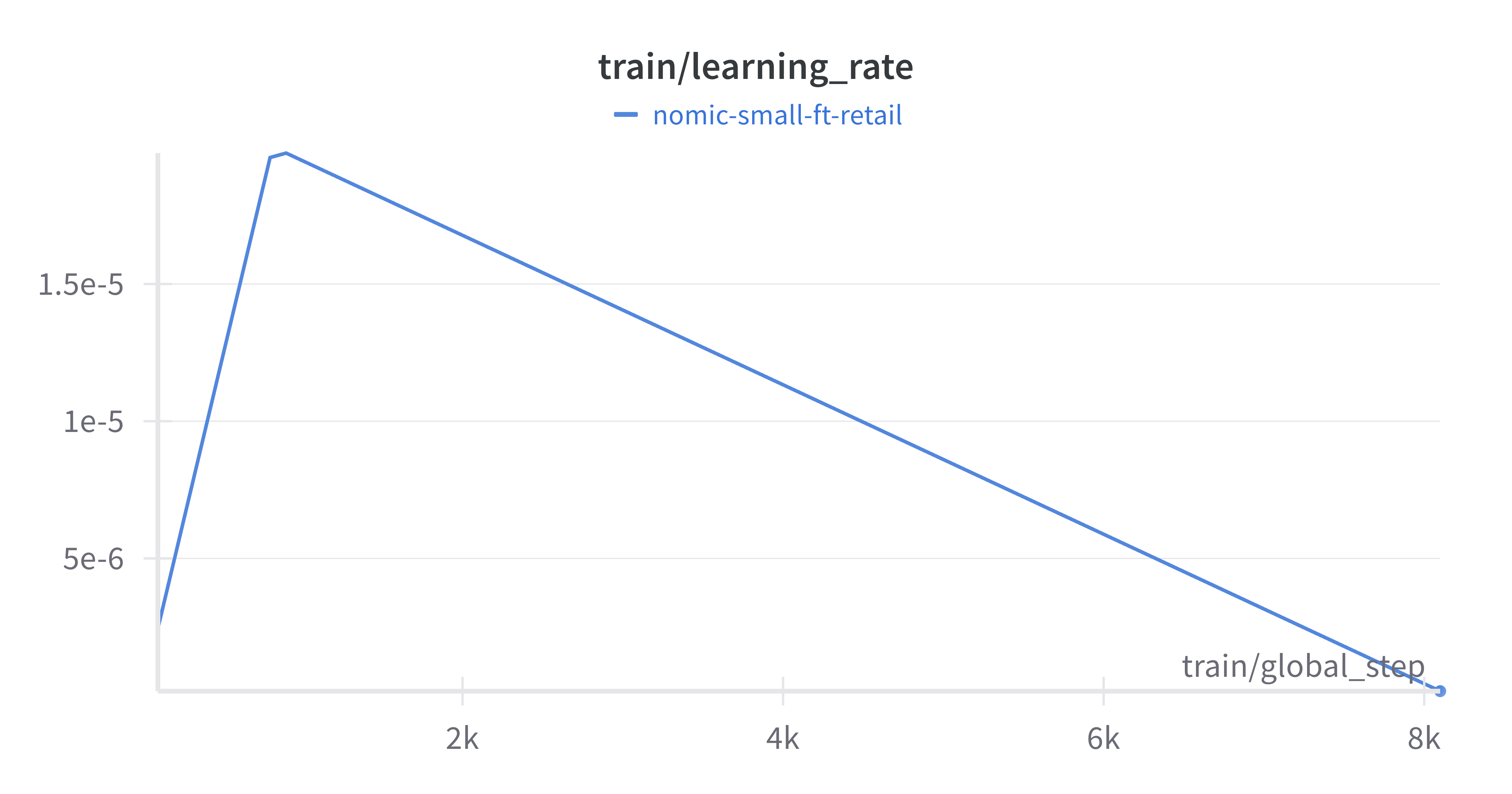
• The initial rise and gradual decay of the learning rate help balance fast convergence and stable learning.
• Provides insight into the optimisation strategy and helps others understand the importance of a dynamic learning rate.

Gradient Norm (train/grad_norm)

This chart tracks the gradient norms, which reflect the stability of the optimisation process.

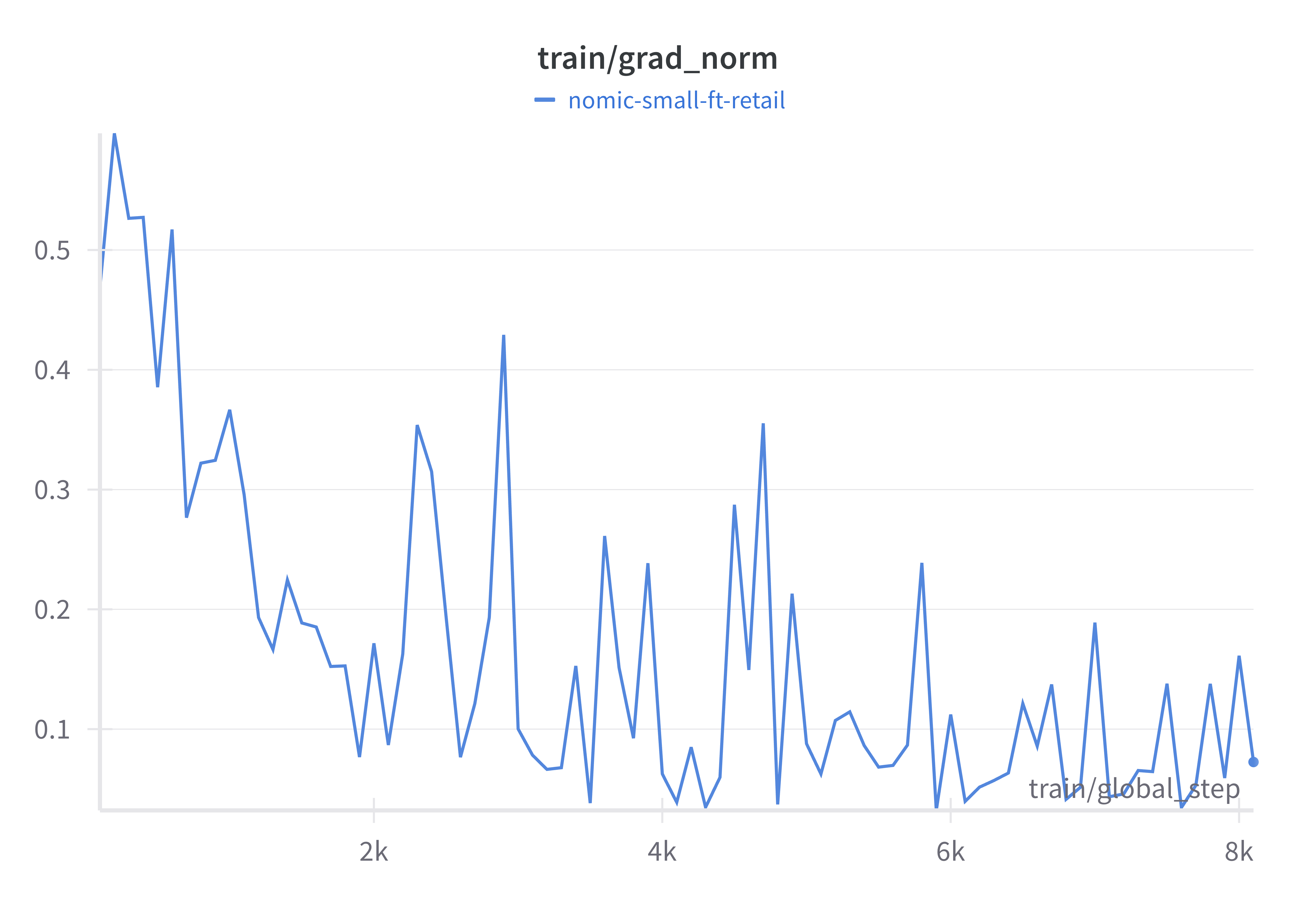
• Stable gradient norms throughout the process suggest that the training avoided exploding or vanishing gradients.
• Useful for debugging and ensuring a stable training process.

Evaluating Model Performance: Fine-Tuned vs. Base Model

After fine-tuning the model, it’s natural to ask:

How much better is the fine-tuned model compared to the base model?

To measure this, we compared the fine-tuned model (FT_model) with the original base model (base_model) using a dedicated test dataset.

This section is all about walking you through how we evaluated both models, what we found, and why it matters.

The Benchmark Dataset

To test the models, we carefully curated the test dataset that we will be using to evaluate and compare the performance contains 21,758 rows, each with:

• sentence1: The first sentence in a pair.
• sentence2: The second sentence in a pair.
• score: A similarity score, representing human-labeled similarity between the two sentences (ranging from 0 to 1).

This dataset serves as our benchmark for evaluating the semantic understanding of both models.‍

Dataset({
    features: ['sentence1', 'sentence2', 'score'],
    num_rows: 21758
})

1. Initialising the Models

Both models were initialised using the SentenceTransformer class from the Sentence Transformers library. The fine-tuned model was specifically trained on retail product data, making it specialised for the task, whereas the base model was a general-purpose model without task-specific adjustments.

Here’s how we set up the models:

from sentence_transformers import SentenceTransformer

# Initialize the fine-tuned model
FT_model = SentenceTransformer("mavihsrr/bge-final-small-retail-v2")

# Initialize the base model
base_model = SentenceTransformer("BAAI/bge-base-en")

Both models were tested on the same dataset to ensure a fair comparison.

2. How We Evaluate Model Performance(The Metrics)

To evaluate the models, we used the EmbeddingSimilarityEvaluator from Sentence Transformers. This tool calculates how similar the embeddings (vector representations) of two sentences are and compares them to the human-labeled similarity scores.

EmbeddingSimilarityEvaluator requires the following inputs:

• sentences1: A list of sentences (from sentence1) to encode.
• sentences2: A list of corresponding sentences (from sentence2) to compare.
• scores: Ground truth similarity scores.

We set it up like this:

from sentence_transformers.evaluation import EmbeddingSimilarityEvaluator, SimilarityFunction

test_evaluator = EmbeddingSimilarityEvaluator(
    sentences1=test_dataset["sentence1"],
    sentences2=test_dataset["sentence2"],
    scores=test_dataset["score"],
    main_similarity=SimilarityFunction.COSINE,  # Uses cosine similarity for comparison
    name="dev"
)

Why EmbeddingSimilarityEvaluator?

This evaluator is designed for tasks involving similarity scores, such as product matching, recommendation systems, and taxonomy fixes. It outputs evaluation metrics to quantify how well the model predicts the relationship between sentence pairs.

Sentence Transformers provides additional evaluators like BinaryClassificationEvaluator for binary labels, which may suit different tasks. You are encouraged to explore these options based on their dataset format and use case.

The evaluator outputs two correlation metrics:

Pearson Correlation: It is crucial for tasks requiring absolute similarity scores, such as product clustering or grouping.

• Measures the linear relationship between predicted similarity scores and actual scores.
• A high Pearson score indicates that the model's predictions align closely with ground truth on a continuous scale.

Spearman Correlation : Ideal for tasks where ranking matters, such as search relevance or recommendations.

• Evaluates the rank-based relationship between predicted and actual scores.
• Focuses on whether the model ranks pairs in the same order as humans do.

Think of Pearson as “How close are we to the actual score?” and Spearman as “Are we ranking things correctly?”

3. Comparing Results

We evaluated both models on the test dataset using the evaluator. Here are the results:

Interpretation of Results:

• Base Model:
  • Pearson: With a score of 0.528, the base model struggles to align its predictions with human-annotated scores.
  • Spearman: A score of 0.469 indicates difficulty in ranking pairs consistently with human intuition.
• Fine-Tuned Model:
  • Pearson: The fine-tuned model achieves an almost perfect score of 0.991, demonstrating a remarkable ability to align with ground truth.
  • Spearman: A score of 0.705 shows that the fine-tuned model ranks sentence pairs more effectively.

4. Real-World Comparison

Accurately identifying the similarity between products is more critical than it might seem. To test how fine-tuning an embedding model can improve similarity detection, we compared the results of a fine-tuned model against a base model using a variety of real-world product descriptions.

We selected a range of product pairs that were challenging but common in retail. These products were either similar in description or fell within the same category but had subtle differences. Here are the pairs we tested:

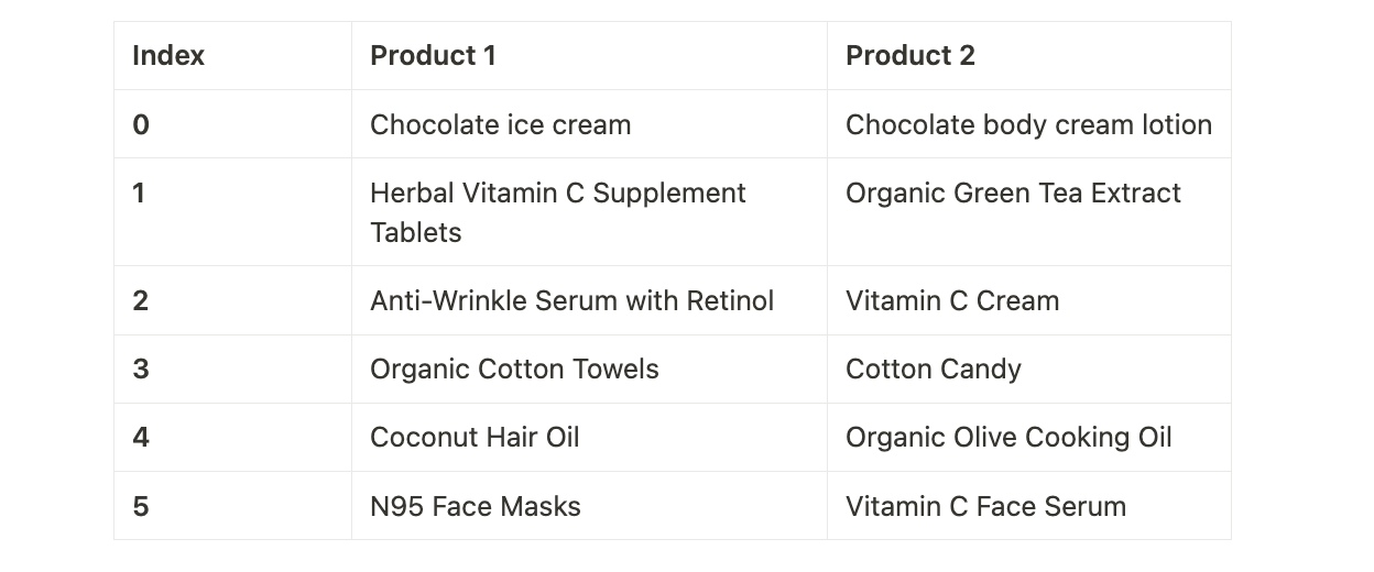
These pairs are tricky because, even though they might seem similar, each product has its own specific use or category. For example, “Coconut Hair Oil” and “Organic Olive Cooking Oil” are both oils, but one is meant for hair care while the other is a cooking ingredient. Identifying these subtle differences is important for businesses that need to categorize products correctly.

What We Did: Calculating Cosine Similarity

To measure how well each model understood the relationships between these pairs, we used cosine similarity. This is a method for calculating how close two product descriptions are to each other in terms of meaning.

We ran both the base model (pre-trained without fine-tuning) and the fine-tuned model (trained on a retail-specific dataset) on these sentence pairs. The results? The fine-tuned model outperformed the base model across almost every pair.

The Results: Base vs. Fine-Tuned Model

Here’s a summary of the results from the two models:

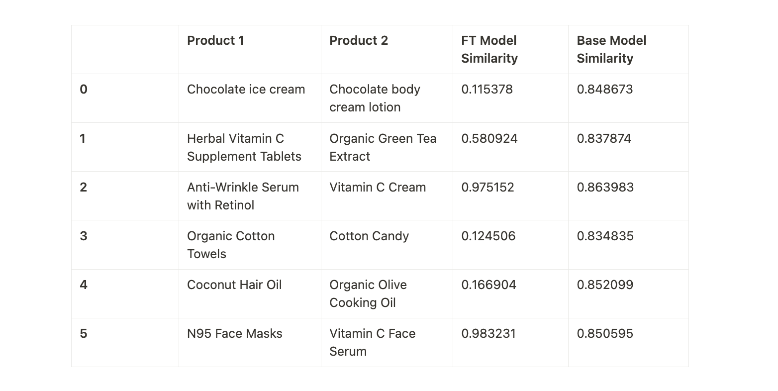
The fine-tuned model was able to distinguish between similar-sounding products and returned accurate similarity scores, particularly in cases where the base model failed. For example, the pair "Chocolate ice cream" vs "Chocolate body cream lotion" has a very low similarity score of 0.115378 from the fine-tuned model, which correctly indicates that these two products are very different in nature. On the other hand, the base model gave a surprisingly high score of 0.848673, incorrectly suggesting a strong similarity between them.

The base model, which was not fine-tuned for specific retail use cases, struggled to understand the nuanced differences between products, often giving unexpectedly high similarity scores for products that were clearly different. For example, the pair "Herbal Vitamin C Supplement Tablets" and "Organic Green Tea Extract" returned a high similarity of 0.837874 from the base model, despite the products having different uses (a supplement vs a tea extract). The fine-tuned model, however, scored them 0.580924, showing it had a better grasp of their distinction.

Why This Matters for Your Business

Whether you’re leading a retail organisation, managing e-commerce operations, or overseeing AI-driven product development, the implications are significant. The fine-tuned model’s superior performance directly translates to business value.

1. Better Search Results: Traditional search engines often rely on exact keyword matching or basic text similarity. This approach struggles to understand the context or intent behind a query, leading to irrelevant search results.Solution?A fine-tuned model, however, understands the semantics of queries. For instance, if a customer searches for "light cotton shirts for summer," it surfaces relevant products—even when the exact phrase doesn’t match—such as “breathable cotton polos” or “linen-blend tees.”The impact?
   • Customers quickly find what they need, improving satisfaction and boosting sales.
   • A seamless search experience encourages repeat visits.
   • Offering smarter search sets you apart in a competitive landscape.
2. Smarter Recommendations: Generic recommendation systems often fall short, especially when user data is sparse or product categories are highly diverse. Fine tuned embeddings bridge this gap by identifying deep, meaningful relationships between products.For example, the model might recommend a “leather laptop bag” to a customer browsing for “formal office shoes,” understanding the professional use case common to both products.
3. Accurate Categorisation: As product catalogs grow, maintaining an accurate taxonomy becomes a daunting task. Misclassifications can confuse customers, slow down searches, and disrupt inventory processes.With the usage of a better model, like our fine tuned model in this case, product descriptions are analysed contextually, ensuring precise categorisation. This model can also seamlessly migrate legacy taxonomies to new ones, aligning your data with current operational needs.
4. Why this matters:
5. • Reduces manual effort in product classification, saving time and resources.
   • Correctly categorised products make it easier for customers to find what they need.
   • The system effortlessly adapts to growing catalogs or evolving taxonomies.
6. Improved Inventory Management: Efficient inventory management often relies on correctly grouping similar products, a process traditionally driven by manual intervention or rigid rules. Such methods are prone to errors and inefficiencies.The fine-tuned model simplifies this by clustering similar products intelligently. For instance, it might group “stainless steel water bottles” with “insulated thermos flasks” based on their use cases, rather than relying on simple product titles.

What's Next?

As we've seen, experimenting with training parameters, whether that means adjusting the number of epochs, modifying learning rates, or altering other hyper parameters based on the dataset, can lead to even better results. There's always room for improvement, and tuning these aspects could make your model more tailored and efficient.

Next steps : Looking ahead, the next logical step is to scale. Moving to a larger model with 500M+ parameters will likely provide more nuanced and refined outputs, thanks to its increased capacity for handling complex patterns in data. While we’ve made progress here, the goal is to continue refining, experimenting, and scaling to unlock even more potential in our AI systems.

If you’re looking to create custom AI solutions that solve specific problems or need help refining your models, feel free to reach out to us.

Thanks for reading :)